Notes on writing a voxel game in Dyalog APL

• 06 March 2026
• apl,
• game dev,
• graphics

Introduction

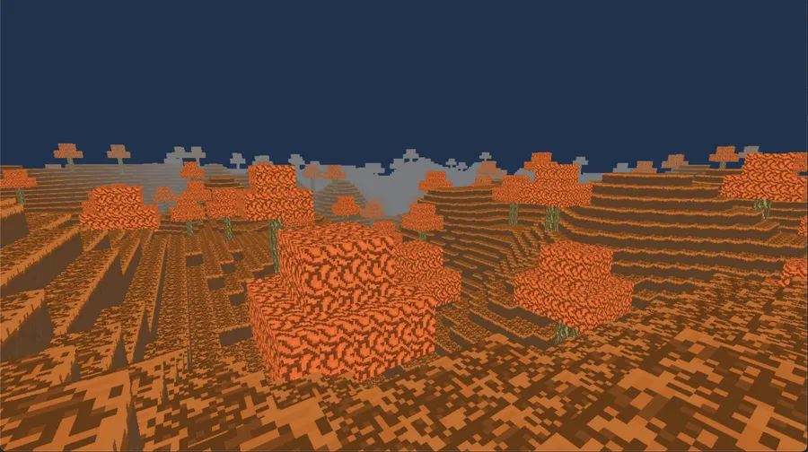
Since November 2025 I have been writing a voxel game in Dyalog APL.

You can see its Github here alongside this and that video demo of me playing around with it.

While there is still more to do, I have reached the point where I am able to describe my experience doing this as someone who has only started learning APL since August 2025.

If you didn't know, APL is a programming language developed by Kenneth Iverson in the 60s and implemented in IBM. It is known for being concise, having arrays as first-class citizens and having non-ASCII symbols for its core functionality (primitives). Primitives can be applied on arguments of arbitrary dimensions.

For example:

	1 + 1
2
	⍝ A 2-by-2 matrix 
	⊢M←[1 2⋄3 4]
1 2
3 4
	1 + M
2 3
4 5
	⍝ Sum-reduce
	+/1 2 3 4 5
15
	⍝ Sum-reduce by rows
	+/M
3 7
	⍝ Sum-reduce by columns 
	+⌿M
4 6

With primitives focused on different ways of moving the data and looking through it, code that would take a lot of lines can be significantly reduced down at the expense of being more terse to the average onlooker.

A famous example frequently shown is Conway's Game of Life in APL, which fits into one line:

life ← {⊃1 ⍵ ∨.∧ 3 4 = +/ +⌿ ¯1 0 1 ∘.⊖ ¯1 0 1 ⌽¨ ⊂⍵}

Proponents of APL will argue that its tersity allows for quick iteration and relieving your thought process from expression and letting it focus on the problems themselves. Critics will point to how it's a write-only language that is unreadable and hard to maintain.

I am someone who prefers to chew my own gum and not let other people chew it for me, so after stumbling upon a Tetris implementation in APL and seeing many claims of the benefits of APL by Aaron Hsu, I realized that APL's notation would provide an interesting way to make a voxel game. Thus, I set out on learning APL so that I could implement something like this and see what writing a complex system in APL is like.

Overview

Briefly, the goal was to implement something similar to Minecraft, which splits its world map into numerous chunks of blocks of the same size. These chunks are vertically limited but repeat cardinally for a long distance. This format fit in perfectly with APL. For this project, the chunks were given sizes of 16-by-128-by-16.

This was written in Dyalog APL 20.0. With Dyalog's functions for calling C libraries, I utilized SDL3 for window management, SDL3_ttf and SDL3_image for fonts and images and SDL's new GPU library, which provided a low level wrapper around many modern graphics apis.^[1] Additionally, I wrote a wrapper for many operations that work with SDL3 that would be painful to express in APL. The wrapper encompassed stuff like this:

1. SDL uses a union headed by an enum for event polling (checking key presses, mouse movement, closing the window). I don't think would be possible to properly express tagged unions in APL without massive pain. Instead, I wrote functions that checked if keys were pressed, the mouse was moved and functions that returned relevant data if these events did happen.
2. SDL's SDL_GPUGraphicsPipelineCreateInfo is expected as a pointer argument to SDL_CreateGPUGraphicsPipeline and has many structs as references in its fields. From experimenting, I do not think that defining structs as reference in structs used as reference is possible in Dyalog's foreign function library, so I split up the creation of the pipeline into numerous chunks.
3. SDL3_ttf uses linked lists for iterating on text to render them. This would have been painful to do in APL in comparison to handling it in C.

After writing bindings for the subset of relevant SDL3 functions I needed, these questions were considered:

Can APL (and can I):

• Convert internal chunk data to vertex data (a format that allows them to be rendered)?
• Perform culling so that only chunks that are seen by the camera are rendered?
• Do collision detection against chunks so that the player can move around the world?
• Do ray testing so that a player can place and break blocks?
• Do basic terrain generation at a constant rate?
• Load chunks in and out of memory constantly as the player moves around the world?

And most importantly, do everything listed here while maintaining at minimum 60 frames per a second as close as I can get to the "APL way"

The Answer: yes

To showcase this, I will outline converting chunk data to positions that are passed to the GPU.

Converting chunk data to vertex data

Given a 3d array, we need to convert it to a format where each solid block is turned into the points of various triangles so that the chunk can be rendered.

⍝ At Initialization
l ← 16 128 16
box ← ⊃∘.∨/1@0¨l-⍛↑¨1

faces ← [
0 1 0 ⋄ 0 1 1 ⋄ 0 0 1 ⋄ 0 0 0 ⍝ Left
1 1 1 ⋄ 1 1 0 ⋄ 1 0 0 ⋄ 1 0 1 ⍝ Right
1 0 0 ⋄ 0 0 0 ⋄ 0 0 1 ⋄ 1 0 1 ⍝ Bottom
0 1 0 ⋄ 1 1 0 ⋄ 1 1 1 ⋄ 0 1 1 ⍝ Top
1 1 0 ⋄ 0 1 0 ⋄ 0 0 0 ⋄ 1 0 0 ⍝ Back
0 1 1 ⋄ 1 1 1 ⋄ 1 0 1 ⋄ 0 0 1 ⍝ Front
]
v_cnt ← ≢faces

vertices ← ,[⍳4] faces(+⍤2) v_cnt(⌿⍤2),[2.5] 3 0 1 2⍉l⊤⊢l⍴⍳×/l
indices←,0 1 2 0 2 3∘.+⍨4×⍳4÷⍨≢vertices

⍝ When copying a chunk to a transfer buffer
∇ info←Copy_chunk(chunk ptr offset);flat;solid;edges;exposed;m;vert;tex;buf;vs;ic
	flat←∊chunk
	solid←chunk≠0
	edges←solid∧box
	exposed←↑[0]{edges∨solid>⍵}¨0 1 2∘.{⍵⌽[⍺]solid}¯1 1 
	vert←vertices⌿⍨4/m←∊exposed
	tex←(⍳×/l)(×⍤¯1),[1+⍳2],[⍳3]exposed                  
	tex←∊(⍳6)(+⍤1)6×flat[tex]                            
	tex←4/m/,##.block_data.tex_z[tex]                    
	vert+←(3,⍨≢vert)⍴128×[0 0 0 ⋄ 0 0 1 ⋄ 1 0 1 ⋄ 1 0 0] 
	buf←∊vert,tex
	vs←≢buf
	ic←6×4÷⍨≢vert
	_←##.LSE_MemcpyU8(ptr+offset)buf vs
	info←vs ic
∇

At a glance, the entire function to copy GPU data into memory is 14 lines of code under the function Copy_chunk. This entire function fits onto my screen and I'm able to see everything it does at once.

For a broad overview, the function takes in a 3d array of size 16-by-128-by-16 and converts it into vertex data that is copied to the GPU. To do this, it utilizes data representing all the possible faces of a chunk which is created at the start of the application.

Briefly, APL provides primitives to select elements of vectors or sub-dimensions of multi-dimensional arrays with bit vectors of the same size (if you've worked with numpy and pytorch, this will seem familiar) like this:

	⍝ Get the numbers from 1 to 10
	⊢x←⍳10
1 2 3 4 5 6 7 8 9 10
    ⍝ Is the remainder of the number times 0.5 0?
	(0=1|0.5×x)
0 1 0 1 0 1 0 1 0 1
    ⍝ Get where the number is equal
	(0=1|0.5×x)/x
2 4 6 8 10

It furthermore provides primitives for data transformations on arbitrary-sized arrays like these:

    ⍝ three by three matrix
	⊢x←3 3⍴⍳9
1 2 3
4 5 6
7 8 9
      ⍝ Rotate it by two upwards
      2⊖x
7 8 9
1 2 3
4 5 6
	⍝ Transpose it 
	⍉x
1 4 7
2 5 8
3 6 9
	⍝ Rotate it by one to the left
	1⌽x
2 3 1
5 6 4
8 9 7
	⍝ Use a bit vector to select the first and third row of that rotation 
	1 0 1⌿1⌽x
2 3 1
8 9 7

With functions like these being the bread and butter of APL, the process of converting chunks can be formulated as selecting the faces that are visible from data that contains all the possible faces of a chunk

vertices ← ,[⍳4] faces(+⍤2) v_cnt(⌿⍤2),[2.5] 3 0 1 2⍉l⊤⊢l⍴⍳×/l

This snippet creates all possible faces of a chunk and returns it in the format of a 2d array with the number of vertices being rows and positions as columns. While I don't expect you to understand the APL behind this, allow me to try and walk you through to data flow so that you can try and visualize what goes on in your head. APL evaluates right-to-left, so let's start!

For the purposes of visualization, instead of a 16-by-128-by-16 chunk, let's do a 3-by-3-by-3!

We first need to get the number of elements in the array

	×/3 3 3
27

From this, let's get the range of indices!

	⍳×/3 3 3
0 1 2 3 4 5 6 7 8 9 10 11 12 13 14 15 16 17 18 19 20 21 22 23 24 25 26

Instead of this being a flat vector, we can reshape this back into a 3-by-3-by-3 array.

	3 3 3⍴⍳×/3 3 3
 0  1  2
 3  4  5
 6  7  8
        
 9 10 11
12 13 14
15 16 17
        
18 19 20
21 22 23
24 25 26

APL has a neat symbol called encode (⊤) that we can use on this array to go "convert to a different numbering system!" In our case, we want to do a numbering system that is the size of the chunk.

Why? For a more minimal example, encode on a range of 8 numbers on a 4-by-2 array looks like this:

	4 2⊤0 1 2 3 4 5 6 7
0 0 1 1 2 2 3 3
0 1 0 1 0 1 0 1

Each number is translated into a unique integer position on our array! We can extrapolate it to higher dimensions and get all the possible positions that blocks fall into in a chunk.

Doing it on our data, we get the following:

	3 3 3⊤3 3 3⍴⍳×/3 3 3
0 0 0
0 0 0
0 0 0
     
1 1 1
1 1 1
1 1 1
     
2 2 2
2 2 2
2 2 2
     
     
0 0 0
1 1 1
2 2 2
     
0 0 0
1 1 1
2 2 2
     
0 0 0
1 1 1
2 2 2
     
     
0 1 2
0 1 2
0 1 2
     
0 1 2
0 1 2
0 1 2
     
0 1 2
0 1 2
0 1 2

It's a lot, but it doesn't look that informative in comparison to the minimal example.

We are trying to visualize a 4d array in 2d, after all. But let's eyeball the data a bit. From each sub-3-by-3-by-3 array take the first 3-by-3 array.

0 0 0
0 0 0
0 0 0

0 0 0
1 1 1
2 2 2

0 1 2
0 1 2
0 1 2

What happens when you merge the elements of these arrays against each-other?

(0, 0, 0) (0, 0, 1) (0, 0, 2)
(0, 1, 0) (0, 1, 1) (0, 1, 2)
(0, 2, 0) (0, 2, 1) (0, 2, 2)

Looks like our unique positions can be found! We just need to move around the array somehow.

We can rearrange the axes around using dyadic transpose (3 0 1 2⍉) to have the positions appear at the last dimension. I wouldn't try to visualize a 4-dimensional rearrangement of the data, just trust me on this and look at the results.

	3 0 1 2⍉3 3 3⊤3 3 3⍴⍳×/3 3 3
0 0 0
0 0 1
0 0 2
     
<...>
     
1 1 0
1 1 1
1 1 2
     
<...>
     
2 2 0
2 2 1
2 2 2

Now that looks more like it!

Right now we have a 4 dimensional array of all the positions of blocks in a chunk. Let's insert another dimension with the size of one before the positions with ,[2.5] for reasons that will be explained further on.

Using ⍴ to return the shape of our array as a vector, our dimensions are now

	⍴,[2.5]3 0 1 2⍉3 3 3⊤3 3 3⍴⍳×/3 3 3
3 3 3 1 3

Let's call this new dimension we added the "block" dimension.

Remember, we want to get all possible faces of a chunk. Right now we only have all possible positions!

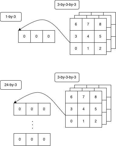
When rendering cubes, each face is dedicated 4 vertices for the four edges of the square of that face. That gives a total of 24 vertices. We set the positions of a cube and its vertex length with the variables faces, in the form of a 24-by-3 array, and vcnt

We can duplicate the block dimension by 24 with v_cnt(⌿⍤2), which really just duplicates the position. Let's check the size.

	⍴24(⌿⍤2),[2.5]3 0 1 2⍉3 3 3⊤3 3 3⍴⍳×/3 3 3
3 3 3 24 3

Here's an attempt at depicting what goes on:

Interestingly, we can add the 24 vertices that make a cube to each sub-array of 24-by-3 under the "block" dimension with just faces(+⍤2)

I can't show you the result of that (it would take a lot of scrolling). Both of these transformations utilize a powerful primitive in APL called Rank (⍤) which helps specify up to which dimensions of an array should the function be done on.

For a minimal example, let's say we store the positions of different entities of a game in a 2d array.

	⊢pos←[6.0 0.7 9.0⋄13.7 8.0 2.3⋄9.8 0 0⋄100 7 8]
  6   0.7 9  
 13.7 8   2.3
  9.8 0   0  
100   7   8  

Let's say that for some reason, they all move by a block. We can use rank on the first dimension to do it to them all at once.

	(1 0 0)(+⍤1)pos
  7   0.7 9  
 14.7 8   2.3
 10.8 0   0  
101   7   8  

Our array is pretty hefty in terms of dimensions, let's flatten down the first 4 dimensions with ,[⍳4]

Doing that gives us a 2d array with a shape of 648-by-3. We now have all the possible faces of a 3-by-3-by-3 chunk in vertex position form!

Let's store that in A for now:

	A← ,[⍳4] faces(+⍤2) v_cnt(⌿⍤2),[2.5] 3 0 1 2⍉3 3 3⊤⊢3 3 3⍴⍳×/3 3 3
	⍴A ⍝ Test getting shape
648 3

But what do we do with this data?

Internally, chunks are stored as 3d arrays with 0 representing air and numbers greater than 0 representing block types (I plan on making negative numbers represent water or non-blocks). We want to represent these blocks as vertices.

Let's test with mock data. Let's say we have a block of type 4 and 8 next to each other in a array of block data, and everything else is air.

	27 ↑4 8 ⍝ Take 27 from 2, rest are filled with 0
4 8 0 0 0 0 0 0 0 0 0 0 0 0 0 0 0 0 0 0 0 0 0 0 0 0 0
	3 3 3⍴27 ↑4 8 ⍝ Form of a 3d array
4 8 0
0 0 0
0 0 0
     
0 0 0
0 0 0
0 0 0
     
0 0 0
0 0 0
0 0 0

We know that each block has 24 vertices. Out of curiosity, what is the size if we flatten this array back and duplicate each element by 24?

	⍴24/27 ↑4 8
648

The same number as the number of vertices of all possible faces. That makes sense. Why does that matter? Well, since we arranged A in such a way that each position is a row and each 24 positions are of a block in a chunk, we can simply select the vertices that would be used by our blocks by turning the flattened array into a boolean vector that we filter A with.

	(24/0≠27 ↑4 8)⌿A
0 1 0
0 1 1
0 0 1
0 0 0
<...>
0 1 2
1 1 2
1 0 2
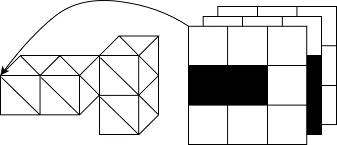
0 0 2

Pretty neat huh? Those are all the vertices we need to render those two blocks in a chunk. Let's say we also do a similar process for getting the colors or uv coordinates of the chunk and we get an array with the same number of rows. For now, each face has the color red. Storing the vertices in B, we can simply just concatenate it to the side like this:

	B←(24/0≠27 ↑4 8)⌿A
	B, [255 0 0⋄]⍴⍨3,⍨≢B
0 1 0 255 0 0
0 1 1 255 0 0
0 0 1 255 0 0
0 0 0 255 0 0
<...>
0 1 2 255 0 0
1 1 2 255 0 0
1 0 2 255 0 0
0 0 2 255 0 0

We can flatten the result and get interleaved vertex data that we pass to the GPU.^[2]

	∊B, [255 0 0⋄]⍴⍨3,⍨≢B
0 1 0 255 0 0 0 <...> 0 0 2 255 0 0

However, those of you observant will note that occluded faces are rendered. That's highly inefficient. Can APL help find a solution to prevent this?

Let's switch back to having chunks that are 16-by-128-by-16. Instead of 648 vertices for all possible faces, we have.. uh.. 786432.

solid←chunk≠0
edges←solid∧box
exposed←↑[0]{edges∨solid>⍵}¨0 1 2∘.{⍵⌽[⍺]solid}¯1 1
vert←vertices⌿⍨4/m←∊exposed

When converting a chunk to vertex data, we want to try and make sure that we only include render visible faces. Rendering faces that are occluded by other blocks would be inefficient, so we only send faces that are exposed in a chunk to the GPU.

A neat way of visualizing how this process could be done in your head is by imagining what happens if you move all solid blocks in one of the 6 directions and comparing that with the original position. If a block intersects with a block when all blocks are moved backwards then that front face of the block isn't visible.

Well, that's what this snippet does!

We:

• Rotate the chunk back and forth on the 3 axes. 0 1 2∘.{⍵⌽[⍺]solid}¯1 1
• Compare the original chunk with each rotation. {edges∨solid>⍵}¨
• Put the comparisons in a form where they're laid out block-by-block. ↑[0]
• Flatten it to be a vector of the same size as number of blocks. m←∊exposed
• Duplicate each element by 4 since each face has 4 vertices. 4/m
• Filter out all the possible faces with this vector. vertices⌿⍨4/m

If you are able to understand everything that has occurred here in terms of data transformation, congrats, you have understood the gist of this APL code. What would take upwards of dozens to a hundred lines of code to do in other languages takes a handful in APL. It furthermore aligns to how I visualize the chunks being transformed into vertex data in my head, which is a nice bonus :-)

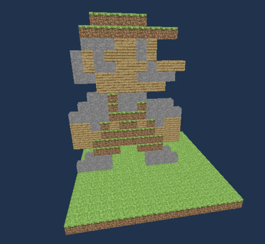
One of the first things I did with this was to render a chunk with Mario on it to see it working.

A lot of the core elements that make up this voxel game are written in this concise style: ray-casting through a grid for placing and breaking blocks, value noise terrain generation, player collision detection, frustum culling and a lot more. This leads to significantly shorter code that I am able to navigate through better.

For instance, the current file to manage everything world related, e.g., frustum culling and drawing, terrain generation, loading chunks in and out of memory and managing shared vertex buffer pools and fences for chunks loading in and out the GPU, is around 300 lines of code, with a fair amount of those lines being dedicated to working with SDL GPU's low level graphics API. This is fairly powerful, allowing me to keep new features I iterate on in a small number of places, significantly reducing the strain of switching between different contexts to figure out what I need to do.

Concise APL code is also very useful when trying to get help for proper solutions. Having snippets, like the example, containing few intermediary variables, focusing on data transformations and being written in a few lines allows me to cut segments from my pipelines and present them to people for possible optimizations. Most of the time, they don't even need to know how these segments fit into the broader picture of what I'm doing (Usually just need to specify what data the segments work on and what I expect out of them). The difference between sharing a few lines of code and being able to bounce around possible solutions versus 40 lines that do the equivalent thing is huge, especially when doing it in a chatroom.

Back to the example, attentive readers will note that rotations wrap around the edges. The variable box is an array of the same shape as the chunk length where the edges are solid that prevents the wrap by just ignoring blocks on the edge for this process. This is sub-optimal, but fine for our purposes.

Attentive readers skilled in APL will notice that the outer product rotation 0 1 2∘.{⍵⌽[⍺]solid}¯1 1 is similar to the outer product rotation done in the Game of Life ¯1 0 1 ∘.⊖ ¯1 0 1 ⌽

This is not a coincidence! The process behind rotating chunks and testing those rotations against something was directly inspired by this process in the Game of Life. It was only months later that I realized I stumbled upon one of the characteristics that Iverson considered a good notation to have: Suggestivity

As Iverson writes in Notation as a Tool of Thought

A notation will be said to be suggestive if the forms of the expressions arising in one set of problems suggest related expressions which find application in other problems.

Furthermore, as Aaron Hsu puts it:

The principle says that suggestive expressions suggest new ideas and themes to a reader by encouraging variations to a given expression that may be alternative solutions to the same problem or may be new expressions that address a different problem but that is now understood to have some connection to the previous problem by virtue of the similarity between the solutions expressed as variations of one another.^[3]

The fact that the Game of Life was done in such a concise manner allowed me to grasp more concretely at what it was doing and see that its process could be applied to my problems.

APLers leverage and extend these sort of terse constructs all the time and call them idioms. Sometimes, they are shorter than how they would be written in English. Splitting a string in Dyalog APL would be ' '(≠⊆⊢)str, in comparison to str.split(' ')

Okay funny symbol man, is this all even performant?

Since large amounts of data are being worked on at once without much branching, the Dyalog interpreter utilizes SIMD and other optimizations to keep this things fast. With this code, I am able to maintain high fps on my MacBook while flying around the map at high speeds and loading chunks. People running on older computers with iGPUs have similarly reported fine performance.

If that video didn't convince you, I went ahead and profiled the aforementioned snippets and some other facts about the game.

• The function that generates all the possible faces of a chunk takes on average 3.5 milliseconds. This is only called in the start of the game.
• The process of getting the vertex positions of all exposed faces of a chunk, as done above, takes 0.46 milliseconds.
  • With textures, it takes 1.8 milliseconds (With low hanging fruits in how I handle textures that I haven't even optimized yet).
• Flying around with a view distance of 8 (289 chunks loaded) and using Dyalog APL's Memory Manager Statistics with 2000⌶ shows that the APL interpreter uses on average 22 megabytes of memory.
  • Chunks with a view distance of 8 take 9 megabytes of memory. Dyalog APL will automatically squeeze data into smaller types if the data falls within a certain range. In this case, blocks need byte. I did not have to do anything to have this happen.
  • Testing with a view distance of 16 shows the total memory being used at 47 megabytes and chunks taking 34 megabytes of memory.

All of this is not too shabby for an interpreted language.

Positives

APL puts data in your face

APL's emphasis on concise code with primitives for data manipulation lends to a coding style where minimal abstraction is needed. What would take designing an abstraction over my understanding of the problem can be instead boiled down to working on the data itself with not much in-between. The previous example showcases this. What would previously require interacting with some chunk object and iterating on blocks over dozens of lines of code is simplified to operations on a 3d array.

For another broad example of this, the chunk data for my game is stored in a 4d array, with the shape of the number of chunks loaded-by-16-by-128-by-16. Accompanying this array is a 2d array with the same number of rows with per-chunk information (position, vertex buffer pointer, the number of indices to help when drawing, etc.)

chunks ← 0⍴⍨0,l
cnames ← 'xz' 'vb' 'vb_kind' 'idx_cnt' 'ready'
chunk_info ← 0⍴⍨0, ≢cnames

Instead of having internal data that is modified by a hefty set of functions, I can instead work on these data structures with a handfuls of various few-liners.

For example:

Unloading chunks that aren't in view distance

range←(ax az ⋄ )+,∘.,⍨(⍳1+2×view_distance)-view_distance
old←range~⍨Cg'xz'
chunks⌿⍨←m←~old∊⍨Cg'xz'
set_m←(0≠Cg'vb')∧~m
vb_fenced⍪←¯1,'vb_kind'{⍉↑⍺ ⍵}⍥{⍵/⍨set_m}⍥Cg'vb'
chunk_info⌿⍨←m

This checks what chunk positions aren't in range, the view distance of the player and removes the row indexes of those positions from the chunk information and chunk 4d array.

Chunks reuse different sized pools of vertex buffers. Vertex buffers from the chunk information that aren't null are passed to concatenated to another data structure to be freed back into the pools when the gpu is finished drawing with them.

All of this being one place with the data right in my face allows me to add and modify different features as I need them. While I currently don't save maps to disk, I am able to see what data I need to use and directly leverage my immediacy to it to add it to the above snippet in a line or two.

APL is ridiculously fast to iterate on

Since the data is in your face and the code is concise, you are able to iterate on solutions at quick speeds once you have a proper understanding of the problem domain. Having to write syntactic structure in the form of numerous branching statements and loops, making sure everything fits into place, no longer becomes a hurdle. This grants you more time to think about the data flow of your problem than the expression.

There have been many times where I meandered about how certain things worked during lunch or when working out in my head, only to be able to sit down and implement or fix what I wanted to in a matter of 30 minutes to an hour before bed. Additionally, there have been many times where what I wrote was shoddy as I was half-asleep and I was able to quickly fix it up in the morning.

For example:

Rendering chunks viewed by the camera.

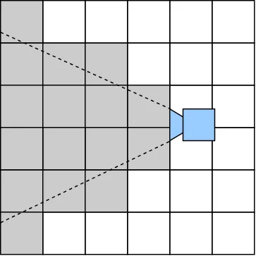
I originally did this by checking whether or not any of the edges of the chunks as viewed from the XZ plane fell in-between the two angles of the camera.

vec←[0 0 ⋄ w 0 ⋄ 0 w ⋄ w w](+⍤2)4/[1],[0.5]↑(⊂px pz-lx lz×w×0.25)-⍨(w←⊃l)×Cg'xz'
dist←0.5*⍨+/[2]vec*2
num←(lx lz)(+.×⍤1)↑vec
den←dist×0.5*⍨+/(lx lz)*2
m←(Cg'ready')∧∨/(○70÷180)>¯2○num(⎕DIV:1).÷den ⍝ Chance that distance could be 0

Showing this to my friend, I realized that this isn't how looking at things work. If one were to take a cone and point it downwards, it would see the stuff behind the person pointing it (Remember the Minecraft Dropper map? :P).

To remedy this, I instead did frustum culling (seeing if points/objects fall inside 6 planes that represent the camera) to test if any of the corner points of the chunk were seen.

frs←##.player.Get_frustum (○70÷180⋄1280÷720⋄0.1⋄500.0)
n←3↑[1]frs
d←,3↓[1]frs
(w h)←(⊃l ⋄ 1⊃l)
box←[
	0 0 0 ⋄ w 0 0 ⋄ 0 0 w ⋄ w 0 w
	0 h 0 ⋄ w h 0 ⋄ 0 h w ⋄ w h w
]
vec←box(+⍤2)8/[1],[0.5]⌽2⌽0,(w←⊃l)×↑Cg'xz'  
t←~(∧/⍤1)(∨/⍤1)0>d(-⍤1)⍨ n(+.×⍤2 1)vec   
t2 ← (2×w)>({0.5*⍨+/⍵*2}⍤1)↑(⊂px pz)-⍨w×Cg'xz'
m←(t2∨t)∧(Cg'ready')

This was written when chunks were 16-by-32-by-16 arrays. Scaling up to a height limit of 128, I quickly realized that this didn't work either. So I found a better solution for AABB frustum culling and implemented it!

frs←##.player.Get_frustum(○70÷180 ⋄ 1280÷720 ⋄ 0.1 ⋄ 500)
n←3↑[1]frs
d←,3↓[1]frs
centers←(w÷2 ⋄ 2÷⍨h←1⊃l ⋄ w÷2)(+⍤1)⌽2⌽0,(w←⊃l)×↑Cg'xz'
r←+/(|n)(×⍤1)(w ⋄ h ⋄ w)÷2
m←(Cg'ready')∧∧/(-r)(≤⍤1)d(-⍤1)⍨n(+.×⍤2 1)centers

Since everything is in one place and I am able to work with the data directly, I was able to quickly iterate on these different solutions to check whether or not chunks were visible or not (usually while half asleep before going to bed). I cannot understate how this surprised me, given that similar experiences in doing this in Rust or C++ required a lot of writing down the structure to pin down what I wanted in dozens of lines of code.

APL is malleable

The usage of idioms, data in your face and quick iteration all come together to allow you to give the feeling that you're playing with your data like it's play-doh. This is only increased due to how Dyalog's IDE, RIDE, works. You are able to have a window open as the REPL and are able to load in your code and edit it. When the code is loaded in and when you edit and save it, you're able to play around with your data.

This creates the feeling of having something akin to a scratchpad to draw out and mess with the data to see what's possible. When I want to implement something, I usually test doing it on mock data in the REPL before testing it in the game. This ability is addicting and makes playing around with your data to figure out possible solutions engaging.

After all, APL was made to write mathematics on the blackboard more easily.

Criticisms

The learning curve is a cliff

I got the idea to make a voxel game in APL in August and only started working on it in November. I spent time going through the numerous online resources for APL in-between those two months, learning and chewing how exactly I could do what I want to do in APL in bite sized pieces. Even now, I don't feel like I have a great handle on a lot of APL's features.^[4]

A native or experienced APLer will point out that most people (me included) only have had experience in ALGOL-influenced languages up until they have seen APL. While that may be true, I am not sure if that would persuade someone to learn an entirely new programming paradigm to be able to appreciate programming in it.

If you aren't paying attention you will suffer

I can divide what I worked on in this game into two distinct moods:

1. I care about how I tackle the problem domain and how I express its solution in APL.
2. I don't really care. I want to get something up and running so I can focus on the parts that I find fun.

A common opinion is that APL is write-only and unreadable. I found that for what I cared about, it was as readable as if I did it in any other programming language, even after coming back to it for a while.

For what I didn't care about (e.g., FFI helper functions, loading SDL3 constants instead of relying on magic numbers), I usually didn't care about implementation and went sprinting to find a solution that worked so I could move on. I found myself quickly forgetting how it worked when returning upon it after months of leaving it be.

While this is something present in other languages, it's easily accelerated in APL and I can imagine it easily screwing someone up. Experienced APLers could say that this is an indication that your solution was ill-formatted and it's a sign to start back up again. Perhaps this is true, since I wrote a lot of this functionality in my early stages of learning APL.

Not all problems can be done well in APL

APL feels excellent where it works well. However, there are edge cases where I feel like it struggles in comparison to a language I would be used to using.

Two examples are handling light and water. If I want to do it in a classic style, I would have to make a 'light map,' where the surface or points like torches would have to breadth-first search crawl in all directions and be blocked by solid blocks. Similarly, working with waters would require knowing specific places in a chunk and seeing whether or not it spreads downwards from those places or not every tick. Solutions to these two problems require functions over the entire 3d array, which I find to feel off, or venture into territory where the APL paradigm falls apart and creates 'code smell'^[5]

The solution to this may be to write the equivalent C functions to handle these problems or to use compute shaders, but I can't help but feel like I am cheating on my initial premise by doing either.

(nitpicky) No floats!?!

The popular array languages currently don't use floats (32-bit, single precision) and instead use doubles (64-bit, double precision). If you've somehow been convinced to try graphics programming or game development in APL from this blog post, you should keep this in mind.

This isn't as much as an issue to me since I pack vertex data into bytes with the format of SDL_GPU_VERTEXELEMENTFORMAT_UBYTE4. Even when I used doubles previously, they only existed when copying chunks into the GPU (Dyalog will convert them to floats if they're passed to a C function that takes floats). However, if you're doing anything that would require having data that would usually be stored as floats in memory (maybe for updating every frame?), then this might be an issue.

A blast from the past

Learning Dyalog APL and working around with it is like stumbling upon an alternate reality where some programming conventions are consistent with current times and some have stayed the same since the 80s. While they have done tremendous work into modernizing it (Not easy keeping an implementation made in the 80s up to date!), one can't help but feel like one has one foot in the modern day and another foot in an era where people still use timeshare systems when playing around with Dyalog APL.

Some interesting tidbits:

• I was evaluating whether to use wgpu-native or SDL GPU with APL early on. Finding out that wgpu-native used callback functions for parts of its API, I investigated the state of callback functions in Dyalog APL. I found out that callback functions are limited to a specific FORTRAN library (I chose SDL GPU after that).
• It seems like there were no source files for most of Dyalog APL's history. Instead, images held code and variables. You would pass them around to work with other people. While there are features such as LINK nowadays that make this irrelevant, one can stumble upon forum posts on how to share or run code with images in bewilderment.
• Dyalog APL was created before unicode was a thing. Yeah. This wasn't a concern for me, since they now use unicode, but it seems like there's still builds of Dyalog APL that don't use unicode for compatibility reasons.
• Lots of functionality that indicate a long history. ⎕OFF exits the program, seems like back then it would turn off the machine APL runs on. There's a system function ⎕ML to switch some APL primitives to do what they would do in a different APL implementation. And of course, setting the index origin to 1 or 0 with ⎕IO.

I find most of this fun, I enjoy learning about the history of why things ended up like this versus that. However, I can imagine someone coming into APL and getting disorientated seeing stuff like this. And of course, these issues aren't in newer array languages such as BQN or Uiua.

Conclusion

APL was a joy to go from nothing to where I am now. This project felt extremely rewarding to work on, it was stimulating to figure out how to handle things I only knew how to do traditionally. I plan on continuing to work on it and seeing how many features I can add, probably targeting Perlin noise and saving maps next.

There's a lot more I want to explore:

• Right now, this has only been me working alone while integrating snippets and improvements other people have recommended. I would like to try reading pre-existing APL code and working with it to see what the process is like when it's not just yourself (Currently reading through Aaron Hsu's dissertation to do this).
• The current algorithms and data of this project are very amenable to being understood through APL. I would like to experiment in more novel techniques that require more thought to properly express in APL. A good example would be modifying Apter trees^[6] to work with quadtrees to implement stuff like this.

So stay tuned!

I recommend trying out APL, or languages in its family, like J, K, BQN and Uiua, for yourself. It proves to be an interesting experience to see how programming could be done so differently to how you're used to doing it.